Outline Eight - Costs and the Firm

Reading Assignment:  None

Remember the old saying, "buy low, sell high" - well this section concerns the part about buying low.  Cost management is very important to any business. 

So let's first review some basic cost comparisons:

Recall from  your principles class the difference between accounting profit and economic profit --

    Total Revenue

-       Explicit or Accounting Costs

=      Accounting Profit or Loss

-       Implicit or Opportunity Costs

=     Economic Profit or Loss

So zero economic profit means that the owners of the firm are just making their opportunity cost. 

This is also known as the normal rate of return.

All economic costs include opportunity costs or payments to the owner of the firm.

The Relationship of Production Functions to Cost Functions. To provide some context for this discussion, consider the problem of producing blueberry pies in my house.  We may have the following relationship.

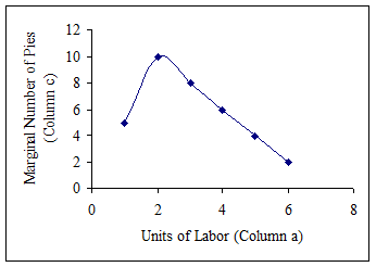
Earlier we focused on short run production - relationship between the number of workers (column a) and the marginal productivity of those workers (column c).  A closely related question pertains to the relationship between the number of pies made (column b) and the marginal costs of making pies (column d).

-After exhausting gains from specialization the relationship between units of labor and marginal productivity is inverse.  This demonstrates the MP of labor curve we looked at earlier.

- Conversely, the marginal cost curve first falls, and then, upon exhausting gains from specialization, increases. So it's basically the opposite of the MP curve.

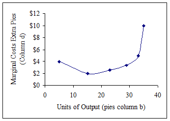
- Intuitively, marginal costs increase as Marginal productivity decreases, because as marginal productivity decreases, this implies that more labor is “imbedded in each unit of output" - we don't get as much out of our inputs, so to produce the same amount, we need more of them, MC increases.

In this section we focus on the relationship between inputs and outputs (MC and outputs). 

We start with the single output case, first in the short run, and then in the long run.  Then we consider some aspects of costs in a multi-product firm.

Short Run Costs.  Recall that the short run is defined as a timeframe where there are both fixed and variable inputs. 

The short run cost function may be used to describe this relationship.

Cost function components - Review:

Fixed costs:  Costs associated with fixed input commitments.  These costs do not change with the level of output

Variable costs:  Costs associated with the variable components.  These costs vary with the level of output.

Total cost relationships. One way to represent these costs is in terms of total expenditures. 

Assumptions:

1. Two inputs, labor and capital
2. Short run
3. Single product
4. Technology fixed
5. "Most" efficient
6. Diminishing marginal returns

Let’s shift to a new problem expressed exclusively in terms of Q. Consider, for example, the first three columns of the following table.

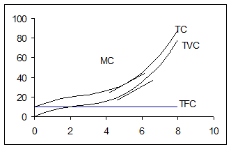
Graphically, these relationships appear as follows:

-Notice that the TVC and the TC curves both take on the shape of a “recliner”: that is, first increasing at a decreasing rate, and then increasing at an increasing rate.  Why?  Div and Specialization (increasing at a decreasing rate) and then Diminishing Marginal Returns (increasing at an increasing rate).

The difference between the two curves is TFC, which is a fixed amount.

Remember too: That MC is change in TC so it is also the slope of the line tangent to either TVC or TC. 

Marginal costs first decrease and then increase due to the law of diminishing returns.  (This is the same logic as diminishing marginal productivity or returns:  At the outset, gains from division of labor increase.  Thus marginal productivity increases, and marginal costs decrease, reflecting gains from specialization.  Later, as the law of diminishing returns sets in, marginal productivity falls, as marginal costs increase. Intuitively, more labor is “imbedded” in each unit of output.)

Average Cost Relationships.  The same relationships can be generated by dividing costs by quantity, to get per unit costs.  In this case:

            AFC    =          TFC/Q             (Average Fixed Costs)

            AVC    =          TVC/Q            (Average Variable Costs)

            ATC    =          TC/Q               (Average Total Costs

            MC      =          ΔTC/ΔQ

These are illustrated in the rightmost columns of the above table.  Graphically, these curves are represented as

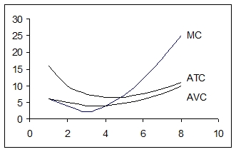
- MC intersects ATC and AVC at their minimum points.  This follows for the same reason that MP intersects AP at its peak:  The marginal drives the average.  The averages reflect the same information as the marginal. 

Let's Again Review The Short Run Shut Down Decision: 

The price a firm might receive for producing units is often dictated by factors beyond the firm’s control. 

 However, suppose that price is fixed.  So that means that P = Average Revenue (AR).

Question:  Why will a firm shut down if unit revenues (AR) do not exceed AVC?

    Because it will be losing more than if it didn't operate and didn't have AVC or AR.  Losing fixed costs either way.

What does breakeven mean in economic terms?

        The firm will breakeven when P or AR = ATC or (TR = TC).

Question:  Why would a firm produce at a loss in the short run?  

    A firm can decrease losses by producing at a loss.  For example, suppose you were a plumber and you had fixed cost obligations of $500 per month for licenses and tool payments. Suppose there was a job that would cost you $1,000 in variable costs to complete (for the month).

    a.  How much must you earn to break even?  Well, TC = $1,500, you would have to earn $1,500.

    b.  How much must you earn to take the job?  Anything over $1,000 - why?

What does breakeven mean in economic terms again?  The breakeven point implies that all factors of production (including the entrepreneur) are earning enough to be indifferent between staying in the industry and doing something else. Firms earn “normal” profits at the breakeven point - or in other words, the owner is just making his or her opportunity cost.

At this point let's graph:  AR or P (assume it is fixed), ATC and MC.

The firm earns zero economic profits at the ATC min, or when AR = ATC

Question:  What would "shift" these cost curves?

Change in technology?

Change in input prices?

How would the curves shift?

Let's Review Our Output Level Decision:

At what level of output will a firm operate to maximize profit or minimize loss?

    Answer:  Where MR = MC  why?

Graph: 

Now, bringing in ATC and AR we can see if the firm is making an economic profit or loss.

If loss -- what will happen in this industry?

If profit -- what will happen in this industry?

Demonstrate all of this on a graph.

Long-Run Costs.  In the Long run, all costs are variable - the firm can change its size.  So the long run may be viewed as the planning horizon, since the project for the firm is to pick the best plant size. Information about the Long-Run Average Cost curve is very useful for determining the structure of an industry (size and number of firms).

Long Run Average Costs.  The long run average cost curve (LRAC) is the envelope of all short run costs curves.  That is, the LRAC is the tangency of all efficient production points on for each plant size.

Graph:

Question:  Where on the graph is Economics of Scale?  Diseconomies of Scale?

                        Economies of scale arise when LRAC falls as the plant expands.

        Reasons for Economies of Scale: 

-         Gains from specialization and division of labor

-         Bulk discounts

                        Diseconomies of scale arise when LRAC increases as the plant expands.

                                Reasons for Diseconomies of Scale

                       -        Transportation Costs (between plants, etc.)

                      -         Bureaucracy with respect to managerial efficiency - red tape.

                        -        Information problems

                        Constant returns to scale - If a range exists where costs neither increase nor decrease.

Minimum Efficient Scale (MES):  The first point where LRAC is at a minimum.

Application:  The shape of the LRAC can determine how many firms can survive in an industry. 

- Suppose that MES is 10,000 units, and that market demand is 40,000 units.  How many efficient firms can survive in the industry?

Multiple Output Cost Functions.  All of the insights pertaining to single product output apply to a multi-product firm.  There are, however some interesting additional cost issues that arise.  Consider, for example, the notion of economies of scope.

Economies of Scope:  Exist when the joint production of two goods is less expensive that the production of both goods separately. 

Economies of scope are an important reason why firms produce multiple products.  For example, it may be more efficient to produce both cars and light trucks in a single plant than to produce both goods separately, the two products may share many parts of the same assembly (such as the chassis) and producing the products separately would mean duplicating of capital equipment unnecessarily.

Cost complementarities:     These exist if the marginal cost of producing one good decreases when the output of another product is increased.  This often arises when one product is a by-product of another. 

Cost complementarities are an important reason for economies of scope.

Note that the existence of economies of scope and cost complementarities have a lot to do with the effectiveness of mergers or the integration we talked about earlier and the sales of subsidiaries.  Sales of an unprofitable subsidiary may not reduce losses much, due to cost complementarities.  Similarly, due to economies of scope, it may be the case that multi-product mergers (conglomerate diversification) are efficient.

Ways to Cut Costs (of course the list could go on and on)...

1.  Supply Chain Management:  

Raw materials - Manufacturing - Transportation - Distribution and Warehousing - Retail Distribution - Consumer

2.  The Strategic Use of Cost:

Example:

3.  Reduction in Cost of Materials: Substitution or Modification

Example:

4. Using Information Technology

Example:

5.  Reduction of Process Costs:

Example:  Use of software instead of paper.

6.  Relocation to lower-wage countries or regions:

Example:  India

7.  Mergers, consolidating and downsizing:

Example: